An RNN (Recurrent Neural Network) model to predict stock price.

• Predicting Stock Price of a company is one of the difficult task in Machine Learning/Artificial Intelligence. This is difficult due to its non-linear and complex patterns. There are many factors such as historic prices, news and market sentiments effect stock price. Major effect is due to historic prices, previous one or many days stock price effects today’s price, hence this is a time series problem. We have chosen Deep Neural Network (RNN) approach to solve this time series (forecasting) problem as it can handle huge volume of data while training the model (when compared with normal Machine Learning models) and the model can be made as complies as possible (thanks to neural networks).
• We have taken IBM stock data from https://www.kaggle.com/borismarjanovic/price-volume-data-for-all-us-stocks-etfs
• Recurrent Neural Networks, tries to understand n – sequential time steps and tries to generate a value close to target value.
• We will implement below RNN architecture we used to solve the problem.

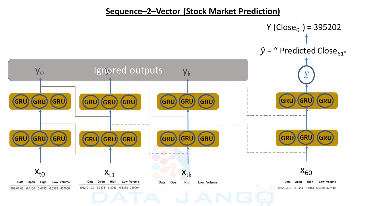
• The Input features are “Date”, “Open”, “High”, “Low” and “Volume”.
• The output/Targe feature is “Close” price.
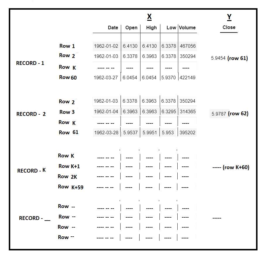
• We will use 60 historic Input Data records(call them as Time Steps) and predict 61st day’s “Close” price. The same is depected in above diagram.

[codesyntax lang=”python”]

import pandas as pd
import numpy as np

import tensorflow as tf

import keras

import matplotlib.pyplot as plt
import seaborn as sns

[/codesyntax]

[codesyntax lang=”python”]

ibm_stock_data = pd.read_csv('../data/ibm_stock_prices.csv')

ibm_stock_data.shape

[/codesyntax]

Output:

(14059, 7)

[codesyntax lang=”python”]

ibm_stock_data.head()

[/codesyntax]

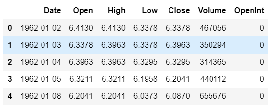
Dropped “OpenInt” as it is not needed

[codesyntax lang=”python”]

ibm_stock_data.drop('OpenInt', axis=1, inplace=True)

[/codesyntax]

Convert date to number

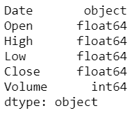
print(ibm_stock_data.dtypes)

[codesyntax lang=”python”]

ibm_stock_data['Date'] = ibm_stock_data['Date'].astype('datetime64')
min_date = ibm_stock_data['Date'].min()
print("min_date : ", min_date)
max_date = ibm_stock_data['Date'].max()
print("max_date : ", max_date)
def calculate_days_since_min_date(row_date):
    return row_date - min_date
ibm_stock_data['numeric_date'] = ibm_stock_data['Date'].apply(lambda x:calculate_days_since_min_date(x))

[/codesyntax]

Output:

min_date :  1962-01-02 00:00:00

max_date :  2017-11-10 00:00:00

[codesyntax lang=”python”]

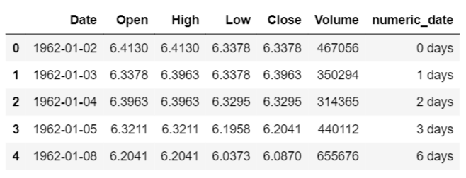
ibm_stock_data.head()

[/codesyntax]

Output:

[codesyntax lang=”python”]

ibm_stock_data.dtypes

[/codesyntax]

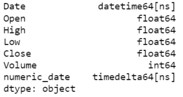
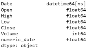
Convert “timedelta64[ns]” to float64

[codesyntax lang=”python”]

ibm_stock_data['numeric_date'] = ibm_stock_data['numeric_date'].astype('timedelta64[D]') 
print(ibm_stock_data.dtypes)

[/codesyntax]

[codesyntax lang=”python”]

ibm_stock_data.drop('Date', axis=1, inplace=True)

[/codesyntax]

Visualize “Closing Price” pattern

[codesyntax lang=”python”]

plt.figure(figsize=(10,10))
plt.plot(ibm_stock_data["numeric_date"], ibm_stock_data["Close"])
plt.title('IBM stock Closeing Price history')
plt.ylabel('Closing Price')
plt.xlabel('Days')
plt.show()

[/codesyntax]

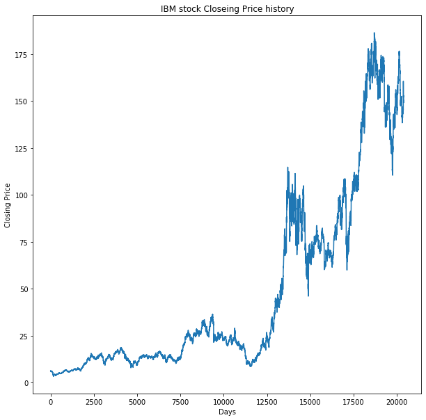
Perform TRAIN/TEST split, we should be doing a sequential split as we are trying to recognize sequential data patterns. We have taken first 13020 records as TRAIN set and last 900 records as TEST (unseen dataset).

[codesyntax lang=”python”]

stock_train_set = ibm_stock_data[ibm_stock_data.numeric_date <= 19000.0]
stock_test_set = ibm_stock_data[ibm_stock_data.numeric_date > 19000.0]

stock_train_set = stock_train_set.iloc[0:13020]
stock_test_set = stock_test_set.iloc[0:900]

X_train_orig = stock_train_set[['Open', 'High', 'Low', 'Volume', 'numeric_date']].values
y_train = stock_train_set['Close'].values

X_test_orig = stock_test_set[['Open', 'High', 'Low', 'Volume', 'numeric_date']].values
y_test = stock_test_set['Close'].values

[/codesyntax]

Scaling all features to felicitate faster convergence of Neural Networks model (Gradient Descent).

[codesyntax lang=”python”]

from sklearn.preprocessing import MinMaxScaler

sc = MinMaxScaler()
X_train = sc.fit_transform(X_train_orig)
X_test = sc.transform(X_test_orig)

[/codesyntax]

Taking 60 time steps to TRAIN and PREDICT. The model needs a 2-Dimensional input and a 1-Dimensional output matrix. Below diagram is a pictorial representation of the concept. build_time_series_data method will we format data in desired format.

[codesyntax lang=”python”]

TIME_STEPS = 60
def build_time_series_data(x, y):
    row_dim = TIME_STEPS
    col_dim = x.shape[1]
    third_dim = x.shape[0] - TIME_STEPS
    print(third_dim, row_dim, col_dim)
    x_time_series_data = np.zeros((third_dim, row_dim, col_dim))
    y_time_series_data = np.zeros((third_dim))
    num_date_corresponding_to_y = np.zeros((third_dim))
    for i in range(third_dim):
        x_time_series_data[i] = x[i:TIME_STEPS+i]
        y_time_series_data[i] = y[TIME_STEPS+i]
        num_date_corresponding_to_y[i] = sc.inverse_transform(x)[TIME_STEPS+i][4]  # as 5th columns in X is the "numeric_date"
    return x_time_series_data, y_time_series_data, num_date_corresponding_to_y

x_train_time_series_data, y_train_time_series_data, train_num_date_corresponding_to_y = build_time_series_data(X_train, y_train)
x_test_time_series_data, y_test_time_series_data, test_num_date_corresponding_to_y = build_time_series_data(X_test, y_test)

[/codesyntax]

[codesyntax lang=”python”]

from keras import Sequential
from keras.layers import GRU
from keras.layers import LSTM
from keras.layers import Dense
from keras.layers.core import Dropout
from keras.layers.core import Flatten
from keras.layers import GRU
from keras import optimizers

from keras import regularizers

[/codesyntax]

[codesyntax lang=”python”]

BATCH_SIZE = 60

t_row_dim = TIME_STEPS
t_col_dim = X_train.shape[1]
t_third_dim = X_train.shape[0] - TIME_STEPS

rnn_model = Sequential()
rnn_model.add(GRU(3, return_sequences=True, input_shape=(t_row_dim, t_col_dim) ))
rnn_model.add(GRU(3, return_sequences=False))
rnn_model.add(Dense(1))
optimizer = optimizers.Adam(lr=0.7)
rnn_model.compile(optimizer = 'adam', loss = 'mean_squared_error')

[/codesyntax]

[codesyntax lang=”python”]

train_predict= rnn_model.predict(x_train_time_series_data)

test_predict= rnn_model.predict(x_test_time_series_data)

total_data_predicted = np.vstack([train_predict, test_predict ])

num_date = np.hstack([train_num_date_corresponding_to_y, test_num_date_corresponding_to_y])

y_close_price_data = np.hstack([y_train_time_series_data, y_test_time_series_data])

[/codesyntax]

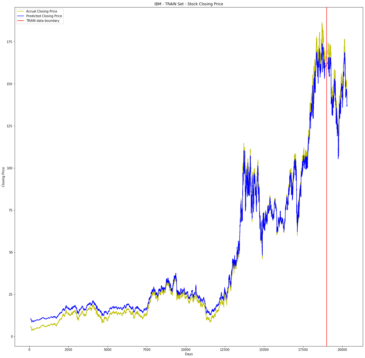
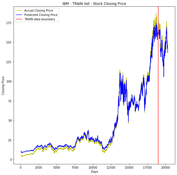
The model is performing very well. In below visualization (Yello – actual close price, Blue – predicted close price), from beginning till 19000 it is TRAIN set, beyond that it is TEST (Unseen) dataset, the model is working well on unseen data as well.

[codesyntax lang=”python”]

fig = plt.figure(figsize=(20,20))
ax = fig.add_subplot(111)
ax.set_title('IBM - TRAIN Set - Stock Closing Price')
#ax.scatter(x=data[:,0],y=data[:,1],label='Data')

plt.plot(num_date, y_close_price_data, color='y', label='Acrual Closing Price')
plt.plot(num_date, total_data_predicted.ravel(),color='b', label='Predicted Closing Price')

#plt.plot(data[:,0], m*data[:,0] + b,color='red',label='Our Fitting Line')
ax.set_xlabel('Days')
ax.set_ylabel('Closing Price')
ax.legend(loc='best')
plt.show()

[/codesyntax]

— By
L Venkata Rama Raju
CEO & Founder
DataJango Technologies Pvt. Ltd.,